HANDOUT
Family of Association Coefficients
(first part
drawn from Zegers, F. E., & ten Berge, J. M. F. (1985). A family of
association coefficients for metric scales.
Psychometrika, 50(1), 17-24 [PDF])
Assume that we are measuring the similarity between vector X and vector Y. We
use X* and Y* to refer to the canonical normalizations (or uniformed versions)
of the X and Y.
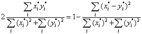
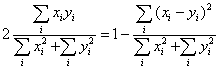
Generic Measure of Similarity
- If X* indicates the uniformed version of X, then Zegers & ten Berge family
of association measures can all be described by the same equation:
Absolute Scale Data
- Identity coefficient. Scale differences not normalized away
- Not mentioned by Z & ten B is the Euclidean distance coefficient. This
measure is not normed -- varies from 0 to ??
Ratio Scale Data
- Tucker's congruence = coefficient of proportionality. Differences in
amplitude normalized away

Additive Scale Data
- Coefficient of additivity = Winer's I
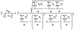
Interval Scale Data
- Pearson correlation = coefficient of linearity
Ordinal data
- Spearman's rho = r(X*,Y*)
- Goodman and Kruskal Gamma = (P - Q)/(P + Q), P is concordant pair and Q is
discordant
- example:
|
|
X |
Y |
|
1 |
1 |
1 |
|
2 |
1 |
2 |
|
3 |
2 |
1 |
|
4 |
2 |
1 |
|
5 |
3 |
1 |
|
6 |
3 |
1 |
|
7 |
3 |
2 |
|
|
1 |
2 |
3 |
4 |
5 |
6 |
7 |
|
1 |
|
n |
n |
n |
n |
n |
p |
|
2 |
|
|
q |
q |
q |
q |
n |
|
3 |
|
|
|
n |
n |
n |
p |
|
4 |
|
|
|
|
n |
n |
p |
|
5 |
|
|
|
|
|
n |
n |
|
6 |
|
|
|
|
|
|
n |
|
7 |
|
|
|
|
|
|
|
P = 3, Q = 4, gamma = -1/7
Or do it via contingency table:
P = 1*(0+1) + 2*(1) = 3
Q = 1*(2+2) +0*(2) = 4
Gamma = -1/7
Another example:
|
City Size/Arenas |
Small |
Medium |
Large |
|
Weak Mayor |
a = 10 |
b = 5 |
c = 2 |
|
Strong Mayor |
d = 10 |
e = 15 |
f = 20 |
P = a(e+f) + bf = 10(15+20) + 5*20 = 450
Q = c(d+e) + bd = 2(10+15) + 5*10 = 100
gamma = (P - Q)/(P + Q) = (450-100)/(450 + 100) = .636
Presence/Absence Data
- Simple matches
- Jaccard
- Gamma / Yule's Q
- (ad-bc)/(ad+bc)
- (OR-1)/(OR+1)
Nominal Data
- (equals phi when table is 2 by 2
|
